Don’t count, predict

In the past couple of years, neural networks have nearly taken over the field of NLP, as they are being used in recent state-of-the-art systems for many tasks. One interesting application is distributional semantics, as they can be used to learn intelligent dense vector representations for words. Marco Baroni, Georgiana Dinu and German Kruszewski presented a paper in ACL 2014 called “Don’t count, predict! A systematic comparison of context-counting vs. context-predicting semantic vectors“, where they compare these new neural-network models with more traditional context vectors on a range of different tasks. Here I will try to give an overview and a summary of their work.

Distributional hypothesis

The goal is to find how similar two words are to each other semantically. The distributional hypothesis states:

Words which are similar in meaning occur in similar contexts
(Rubenstein & Goodenough, 1965).

Therefore, if we want to find a word similar to “magazine”, we can look for words that occur in similar contexts, such as “newspaper”.

I was reading a magazine today	I was reading a newspaper today
The magazine published an article	The newspaper published an article
He buys this magazine every day	He buys this newspaper every day

 

Also, if we want to find how similar “magazine” and “newspaper” are, we can compare how similar are all the contexts in which they appear. For example, to find the similarity between two words, we can represent the contexts as feature vectors and calculate the cosine similarity between their corresponding vectors.

The counting model

In a traditional counting model, we count how many times a certain context word appears near our main word. We have to manually choose a window size – the number of words we count on either side of the main word.

For example, given sentences “He buys this newspaper every day” and “I read a newspaper every day”, we can look at window size 2 (on either side of the main word) and create the following count vector:

[table]
buys,this,every,day,read,a
1,1,2,2,1,1
[/table]

As you can see, “every” and “day” get a count of 2, because they appear in both sentences, whereas “he” doesn’t get included because it doesn’t fit into the window of 2 words.

In order to get the best performance, it is important to use a weighting function which turns these counts into more informative values. A good weighting scheme would downweight frequent words such as “this” and “a”, and upweight more informative words such as “read”. The authors experimented with two weighting schemes: Pointwise Mutual Information  and Local Mutual Information. An overview of various weighting methods can be found in the thesis of Curran (2003).

These vectors are also often compressed. The motivation is that feature words such as “buy” and “purchase” are very similar and compression techniques should be able to represent them as a single semantic class. In addition, this gives smaller dense vectors, which can be easier to operate on. The authors here experimented with SVD and Non-negative Matrix Factorization.

The predicting model

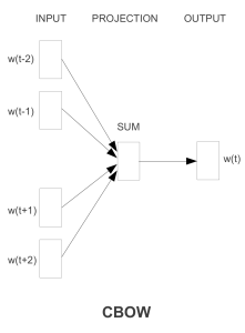
A the neural network (predicting) model, this work uses the word2vec implementation of Continuous Bag-of-Words (CBOW). Word2vec is a toolkit for efficiently learning word vectors from very large text corpora (Mikolov et al., 2013). The CBOW architecture is shown below:

The vectors of context words are given as input to the network. They are summed and then used to predict the main word. During training, the error is backpropagated and the context vectors are updated so that they would predict the correct word. Since similar words appear in similar contexts, the vectors of similar words will also be updated towards similar directions.

A normal network would require finding the probabilities of all possible words in our vocabulary (using softmax), which can be computationally very demanding. Word2vec implements two alternatives to speed this up:

1. Hierarchical softmax, where the words are arranged in a tree (similar to a decision tree), making the complexity logarithmic.
2. Negative sampling, Where the system learns to distinguish the correct answer from a sample of a few incorrect answers.

In addition, word2vec can downsample very frequent words (for example, function words such as “a” and “the”) which are not very informative.

From personal experience I have found skip-gram models (also implemented in word2vec) to perform better than CBOW, although they are slightly slower. Skip-grams were not compared in this work, so it is still an open question which of the two models gives better vectors, given the same training time.

Evaluation

The models were trained on a corpus of 2.8 billion tokens, combining ukWac, the English Wikipedia and the British National Corpus. They used 300,000 most frequent words as both the context and target words.

The authors performed on a number of experiments on different semantic similarity tasks and datasets.

1. Semantic relatedness: In this task, humans were asked to rate the relatedness of two words, and the system correlation with these scores is measured.
   • rg: 65 noun pairs by Rubenstein & Goodenough (1965)
   • ws: Wordsim353, 353 word pairs by Finkelstein et al. (2002)
   • wss: Subset of Wordsim353 focused on similarity (Agirre et al., 2009)
   • wsr: Subset of Wordsim353 focused on relatedness (Agirre et al., 2009)
   • men: 1000 word pairs by Bruni et al. (2014)
2. Synonym detection: The system needs to find the correct synonym for a word.
   • toefl: 80 multiple-choice questions with 4 synonym candidates (Landauer & Dumais, 1997).
3. Concept categorization: Given a set of concepts, the system needs to group them into semantic categories.
   • ap: 402 concepts in 21 categories (Almuhareb, 2006)
   • esslli: 44 concepts in 6 categories (Baroni et al., 2008)
   • battig: 83 concepts in 10 categories (Baroni et al., 2010)
4. Selectional preferences: Using some examples, the system needs to decide how likely a noun is to be a subject or object for a specific verb.
   • up: 221 word pairs (Pado, 2007)
   • mcrae: 100 noun-verb pairs (McRae et al., 1998)
5. Analogy: Using examples, the system needs to find a suitable word to solve analogy questions, such as: “X is to ‘uncle’ as ‘sister’ is to ‘brother'”
   • an: ~19,500 analogy questions (Mikolov et al., 2013b)
   • ansyn: Subset of the analogy questions, focused on syntactic analogies
   • ansem: Subset of the analogy questions, focused on semantic analogies

Results

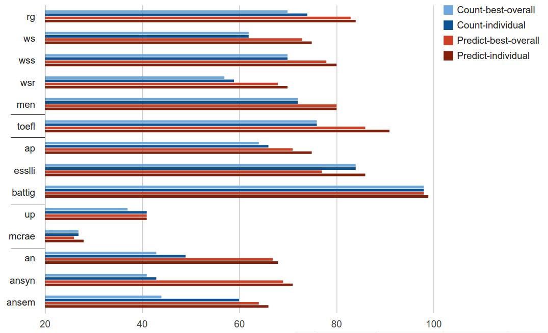
The graph below illustrates the performance of different models on all the tasks. The blue bars represent the counting models, and the red bars are for neural network models. The “individual” models are the best models on that specific task, whereas the “best-overall” is the single best model across all the tasks.

In conclusion, the neural networks win with a large margin. The neural models have given a large improvement on the tasks of semantic relatedness, synonym detection and analogy detection. The performance is equal or slightly better on categorization and selectional preferences.

The best parameter choices for counting models are as follows:

• window size 2 (bigger is not always better)
• weighted with PMI, not LMI
• no dimensionality reduction (not using SVD or NNMF)

The best parameters for the neural network model were:

• window size 5
• negative sampling (not hierarchical softmax)
• subsampling of frequent words
• dimensionality 400

The paper also finds that the neural models are much less sensitive to parameter choices, as even the worst neural models perform relatively well, whereas counting models can thoroughly fail with unsuitable values.

It seems appropriate to quote the final conclusion of the authors:

Our secret wish was to discover that it is all hype, and count vectors are far superior to their predictive counterparts. A more realistic expectation was that a complex picture would emerge, with predict and count vectors beating each other on different tasks. Instead, we found that the predict models are so good that, while triumphalist overtones still sound excessive, there are very good reasons to switch to the new architecture.

The results certainly support that vectors created by neural models are more suitable for distributional similarity tasks. We have also performed a similar comparison on the task of hyponym generation (Rei & Briscoe, 2014). Our findings match those here – the neural models outperform simple bag-of-words models. However, the neural models are in turn outperformed by a dependency-based model. It remains to be seen whether this finding also applies on a wider range of distributional similarity models.

References

Agirre, E., Alfonseca, E., Hall, K., Kravalova, J., Paşca, M., & Soroa, A. (2009). A study on similarity and relatedness using distributional and WordNet-based approaches. Proceedings of Human Language Technologies: The 2009 Annual Conference of the North American Chapter of the Association for Computational Linguistics on – NAACL ’09, (June), 19. doi:10.3115/1620754.1620758

Almuhareb, A. (2006) Attributes in Lexical Acquisition. Phd thesis, University of Essex.

Baroni, M., Barbu, E., Murphy, B., & Poesio, M. (2010). Strudel: A distributional semantic model based on properties and types. Cognitive Science, 34.

Baroni, M., Dinu, G., & Kruszewski, G. (2014). Don’t count, predict! A systematic comparison of context-counting vs. context-predicting semantic vectors. In Proceedings of the 52nd Annual Meeting of the Association for Computational Linguistics (pp. 238–247).

Baroni, M., Evert, S., & Lenci, A., editors. (2008). Bridging the gap between Semantic
Theory and Computational Simulations: Proceedings of the ESSLLI Workshop on Distributional Lexical Semantics.

Bruni, E., Tran, N. K., & Baroni, M. (2014). Multimodal Distributional Semantics. J. Artif. Intell. Res.(JAIR), 49, 1–47.

Curran, J. R. (2003). From distributional to semantic similarity. University of Edinburgh. University of Edinburgh.

Finkelstein, L., Gabrilovich, E., Matias, Y., Rivlin, E., Solan, Z., Wolfman, G., & Ruppin, E. (2002). Placing search in context: the concept revisited. In ACM Transactions on Information Systems (Vol. 20, pp. 116–131). ACM. doi:10.1145/503104.503110

McRae, K., Spivey-Knowlton, M., & Tanenhaus, M. (1998). Modeling the influence of the- matic fit (and other constraints) in on-line sentence comprehension. Journal of Memory and Language, 38:283–312.

Mikolov, T., Chen, K., Corrado, G., & Dean, J. (2013). Efficient Estimation of Word Representations in Vector Space. ICLR Workshop, 1–12.

Mikolov, T., Yih, W., & Zweig, G. (2013b). Linguistic Regularities in Continuous Space Word Representations, (June), 746–751.

Pado, U. (2007). The Integration of Syntax and Semantic Plausibility in a Wide-Coverage Model of Sentence Processing. Dissertation, Saarland University, Saarbrücken.

Rei, M., & Briscoe, T. (2014). Looking for Hyponyms in Vector Space. In CoNLL-2014 (pp. 68–77).

Rubenstein, H., & Goodenough, J. (1965). Contextual correlates of synonymy.
Communications of the ACM, 8 (10), 627–633.