Marek Rei

Political ideology detection

Marek October 5, 2014 Uncategorized 3 Comments

Neural networks have a range of interesting applications, and here I will discuss on one them: recursive neural networks and the detection of political ideology. This post is a summary and analysis of a recent publication by Mohit Iyyer, Peter Anns, Jordan Boyd-Graber and Philip Resnik: “Political Ideology Detection Using Recursive Neural Networks“.

The Task

Given a sentence, we want the model to detect the political ideology expressed in that sentence. In this research, the authors deal with US politics, so the possible options are liberal (democrats) or conservative (republicans). As a practical application we might consider a system that processes a large amount of news articles or public speeches to detect and measure explicit or hidden political bias of the authors.

A traditional approach to this problem is a simple bag-of-words model, where each word is treated as a separate feature, but this ignores any syntactic structure and even word order. As shown below, political ideology can be compositionally complicated – while certain sections of the sentence are locally conservative, the way they are used in context makes the overall sentence liberal.

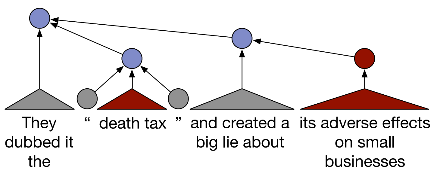
Figure 1: Sample sentence from Iyyer et al. (2014). Blue nodes are liberal, red nodes are conservative, grey nodes are neutral.

Don’t count, predict

Marek September 22, 2014 Uncategorized 5 Comments

In the past couple of years, neural networks have nearly taken over the field of NLP, as they are being used in recent state-of-the-art systems for many tasks. One interesting application is distributional semantics, as they can be used to learn intelligent dense vector representations for words. Marco Baroni, Georgiana Dinu and German Kruszewski presented a paper in ACL 2014 called “Don’t count, predict! A systematic comparison of context-counting vs. context-predicting semantic vectors“, where they compare these new neural-network models with more traditional context vectors on a range of different tasks. Here I will try to give an overview and a summary of their work.

Distributional hypothesis

The goal is to find how similar two words are to each other semantically. The distributional hypothesis states:

Words which are similar in meaning occur in similar contexts
(Rubenstein & Goodenough, 1965).

Therefore, if we want to find a word similar to “magazine”, we can look for words that occur in similar contexts, such as “newspaper”.

I was reading a magazine today	I was reading a newspaper today
The magazine published an article	The newspaper published an article
He buys this magazine every day	He buys this newspaper every day

Also, if we want to find how similar “magazine” and “newspaper” are, we can compare how similar are all the contexts in which they appear. For example, to find the similarity between two words, we can represent the contexts as feature vectors and calculate the cosine similarity between their corresponding vectors.

Neural Networks, Part 3: The Network

Marek February 23, 2014 Neural Networks 1 Comment

We have learned about individual neurons in the previous section, now it’s time to put them together to form an actual neural network.

The idea is quite simple – we line multiple neurons up to form a layer, and connect the output of the first layer to the input of the next layer. Here is an illustration:

Each red circle in the diagram represents a neuron, and the blue circles represent fixed values. From left to right, there are four columns: the input layer, two hidden layers, and an output layer. The output from neurons in the previous layer is directed into the input of each of the neurons in the next layer.

We have 3 features (vector space dimensions) in the input layer that we use for learning: \(x_1\), \(x_2\) and \(x_3\). The first hidden layer has 3 neurons, the second one has 2 neurons, and the output layer has 2 output values. The size of these layers is up to you – on complex real-world problems we would use hundreds or thousands of neurons in each layer.

How to normalise feature vectors

Marek February 8, 2014 Resources 2 Comments

I was trying to create a sample file for training a neural network and ran into a common problem: the feature values are all over the place. In this example I’m working with demographical real-world values for countries. For example, a feature for GDP per person in a country ranges from 551.27 to 88286.0, whereas estimates for corruption range between -1.56 to 2.42. This can be very confusing for machine learning algorithms, as they can end up treating bigger values as more important signals.

To handle this issue, we want to scale all the feature values into roughly the same range. We can do this by taking each feature value, subtracting its mean (thereby shifting the mean to 0), and dividing by the standard deviation (normalising the distribution). This is a piece of code I’ve implemented a number of times for various projects, so it’s time to write a nice reusable script. Hopefully it can be helpful for others as well. I chose to do this in python, as it’s easies to run compared to C++ and Java (doesn’t need to be compiled), but has better support for real-valued numbers compared to bash scripting.

Neural Networks, Part 2: The Neuron

Marek January 25, 2014 Neural Networks 7 Comments

A neuron is a very basic classifier. It takes a number of input signals (a feature vector) and outputs a single value (a prediction). A neuron is also a basic building block of neural networks, and by combining together many neurons we can build systems that are capable of learning very complicated patterns. This is part 2 of an introductory series on neural networks. If you haven’t done so yet, you might want to start by learning about the background to neural networks in part 1.

Neurons in artificial neural networks are inspired by biological neurons in nervous systems (shown below). A biological neuron has three main parts: the main body (also known as the soma), dendrites and an axon. There are often many dendrites attached to a neuron body, but only one axon, which can be up to a meter long. In most cases (although there are exceptions), the neuron receives input signals from dendrites, and then outputs its own signals through the axon. Axons in turn connect to the dendrites of other neurons, using special connections called synapses, forming complex neural networks.

Below is an illustration of an artificial neuron, where the input is passed in from the left and the prediction comes out from the right. Each input position has a specific weight in the neuron, and they determine what output to give, given a specific input vector. For example, a neuron could be trained to detect cities. We can then take the vector for London from the previous section, give it as input to our neuron, and it will tell us it’s a city by outputting value 1. If we do the same for the word Tuesday, it will give a 0 instead, meaning that it’s not a city.

Neural Networks, Part 1: Background

Marek January 19, 2014 Neural Networks 0 Comments

Artificial neural networks (NN for short) are practical, elegant, and mathematically fascinating models for machine learning. They are inspired by the central nervous systems of humans and animals – smaller processing units (neurons) are connected together to form a complex network that is capable of learning and adapting.

The idea of such neural networks is not new. McCulloch-Pitts (1943) described binary threshold neurons already back in 1940’s. Rosenblatt (1958) popularised the use of perceptrons, a specific type of neurons, as very flexible tools for performing a variety of tasks. The rise of neural networks was halted after Minsky and Papert (1969) published a book about the capabilities of perceptrons, and mathematically proved that they can’t really do very much. This result was quickly generalised to all neural networks, whereas it actually applied only to a specific type of perceptrons, leading to neural networks being disregarded as a viable machine learning method.

In recent years, however, the neural network has made an impressive comeback. Research in the area has become much more active, and neural networks have been found to be more than capable learners, breaking state-of-the-art results on a wide variety of tasks. This has been substantially helped by developments in computing hardware, allowing us to train very large complex networks in reasonable time. In order to learn more about neural networks, we must first understand the concept of vector space, and this is where we’ll start.